Let us take a second-order continuous-time linear system: $$\dot{x}(t)=Ax(t), \quad A\in \mathbb{R}^{2\times 2}.$$

For such linear systems, the qualitative behavior of \(x(t)\) is determined by the eigenvalues of \(A\). What makes the \(2×2\) case interesting is that these eigenvalues can be written explicitly in terms of the trace and determinant of \(A\): $$\Lambda(A)= \left\{\frac{\mbox{Tr} A}{2} \pm \sqrt{\frac{(\mbox{Tr} A)^2}{4}-\mbox{det} A} \right\}.$$

Therefore, all qualitative behaviors of these systems can be represented on a \((\mbox{Tr} A, \mbox{det} A)\)-plane. This plane is sometimes called a Poincaré diagram.

In particular, the usual stability condition for continuous-time linear systems (all eigenvalues in the open left half-plane) can be reduced to a simple criteria expressed in terms of \( \mbox{Tr} A, \mbox{det} A\): $$\max\mbox{Re}(\Lambda(A))<0 \Leftrightarrow \max(\mbox{Tr} A, -\mbox{det} A)<0.$$

This condition is particularly useful for control theorists, as it greatly simplifies the characterization of the stabilizing state-feedback gains \(K\) ensuring that a closed-loop system (with \(A_{cl}=A+BK\)) is stable, allowing for quick, back-of-the-envelope calculations.

Although unsurprising, it is rarely brought up that a similar stability condition holds for second-order discrete-time linear systems: $$x_{k+1}=Ax_k, \quad A\in \mathbb{R}^{2\times 2}.$$

Indeed, the usual stability condition (the spectral radius of \(A\) is smaller than \(1\), thus all eigenvalues are in the unit disc) can also be reduced to a simple criteria expressed in terms of \( \mbox{Tr} A, \mbox{det} A\): $$\rho(A)<1 \Leftrightarrow \max( |\mbox{Tr} A| – \mbox{det} A, \mbox{det} A)<1.$$

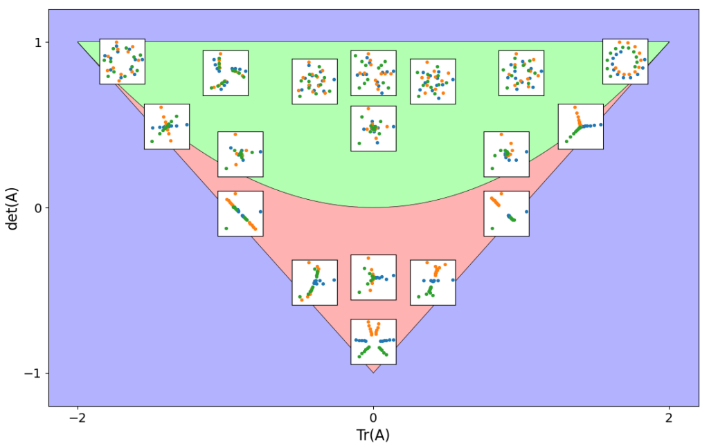
Interestingly, this criterion defines a triangular region on the \((\mbox{Tr} A, \mbox{det} A)\)-plane, sometimes referred to as the ‘stability triangle.’ This triangle is represented hereabove, together with a few sample trajectories produced by systems corresponding to points within it. Analogous to the continuous-time Poincaré diagram, oscillatory behaviors associated with complex eigenvalues occur in the green region, where \((\mbox{Tr} A)^2 < 4\mbox{det} A \). In the red region, only scaling, symmetry flips, and accumulation along eigenvector directions occur.